Data Science - Linear Regression Case
Case: Use Duration + Average_Pulse to Predict Calorie_Burnage
Create a Linear Regression Table with Average_Pulse and Duration as Explanatory Variables:
Example
import pandas as pd
import statsmodels.formula.api as smf
full_health_data = pd.read_csv("data.csv", header=0, sep=",")
model = smf.ols('Calorie_Burnage ~ Average_Pulse + Duration', data = full_health_data)
results
= model.fit()
print(results.summary())
Try it Yourself »
Example Explained:
- Import the library statsmodels.formula.api as smf. Statsmodels is a statistical library in Python.
- Use the full_health_data set.
- Create a model based on Ordinary Least Squares with smf.ols(). Notice that the explanatory variable must be written first in the parenthesis. Use the full_health_data data set.
- By calling .fit(), you obtain the variable results. This holds a lot of information about the regression model.
- Call summary() to get the table with the results of linear regression.
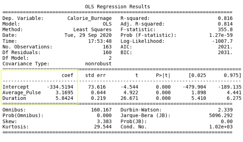
Output:

The linear regression function can be rewritten mathematically as:
Calorie_Burnage = Average_Pulse * 3.1695 + Duration * 5.8424 - 334.5194
Rounded to two decimals:
Calorie_Burnage = Average_Pulse * 3.17 +
Duration * 5.84 - 334.52
Define the Linear Regression Function in Python
Define the linear regression function in Python to perform predictions.
What is Calorie_Burnage if:
- Average pulse is 110 and duration of the training session is 60 minutes?
- Average pulse is 140 and duration of the training session is 45 minutes?
- Average pulse is 175 and duration of the training session is 20 minutes?
Example
def Predict_Calorie_Burnage(Average_Pulse,
Duration):
return(3.1695*Average_Pulse + 5.8434 * Duration - 334.5194)
print(Predict_Calorie_Burnage(110,60))
print(Predict_Calorie_Burnage(140,45))
print(Predict_Calorie_Burnage(175,20))
Try it Yourself »
The Answers:
- Average pulse is 110 and duration of the training session is 60 minutes = 365 Calories
- Average pulse is 140 and duration of the training session is 45 minutes = 372 Calories
- Average pulse is 175 and duration of the training session is 20 minutes = 337 Calories
Access the Coefficients
Look at the coefficients:
- Calorie_Burnage increases with 3.17 if Average_Pulse increases by one.
- Calorie_Burnage increases with 5.84 if Duration increases by one.
Access the P-Value
Look at the P-value for each coefficient.
- P-value is 0.00 for Average_Pulse, Duration and the Intercept.
- The P-value is statistically significant for all of the variables, as it is less than 0.05.
So here we can conclude that Average_Pulse and Duration has a relationship with Calorie_Burnage.
Adjusted R-Squared
There is a problem with R-squared if we have more than one explanatory variable.
R-squared will almost always increase if we add more variables, and will never decrease.
This is because we are adding more data points around the linear regression function.
If we add random variables that does not affect Calorie_Burnage, we risk to falsely conclude that the linear regression function is a good fit. Adjusted R-squared adjusts for this problem.
It is therefore better to look at the adjusted R-squared value if we have more than one explanatory variable.
The Adjusted R-squared is 0.814.
The value of R-Squared is always between 0 to 1 (0% to 100%).
- A high R-Squared value means that many data points are close to the linear regression function line.
- A low R-Squared value means that the linear regression function line does not fit the data well.
Conclusion: The model fits the data point well!
Congratulations! You have now finished the final module of the data science library.
